|
A pair of studies developed and implemented a method to improve the estimates of extreme sea surface temperatures (SSTs) from an eddy-resolving ocean model. First, Oliver et al. (Progress in Oceanography, 2014) developed a Bayesian hierarchical model which uses estimates of large-scale climate statistics (mean, variance, etc) to predict observed extreme SSTs, and then applies the model to a projected future climate. Then, Oliver et al. (Journal of Climate, 2014) applied the model off southeastern Australia and demonstrated that the extreme SSTs in that region are projected to change significantly due to an increase in both the mean SST and the SST variance.
Oliver et al. (Progress in Oceanography, 2014): Estimating oceanic and atmospheric extremes from global climate models is not trivial as these models often poorly represent extreme events. However, these models do tend to capture the central climate statistics well (e.g., the mean temperature, variances, etc). Here, we develop a Bayesian hierarchical model (BHM) to improve estimates of extremes from ocean and climate models. This is performed by first modeling observed extremes using an extreme value distribution (EVD). Then, the parameters of the EVD are modeled as a function of climate variables simulated by the ocean or atmosphere model over the same time period as the observations. By assuming stationarity of the model parameters, we can estimate extreme values in a projected future climate given the climate statistics of the projected climate (e.g., a climate model projection under a specified carbon emissions scenario). The model is demonstrated for extreme sea surface temperatures off southeastern Australia using satellite-derived observations and downscaled global climate model output for the 1990s and the 2060s under an A1B emissions scenario. Using this case study we present a suite of statistics that can be used to summarize the probabilistic results of the BHM including posterior means, 95\% credible intervals, and probabilities of exceedance. We also present a method for determining the statistical significance of the modeled changes in extreme value statistics. Finally, we demonstrate the utility of the BHM to test the response of extreme values to prescribed changes in climate.
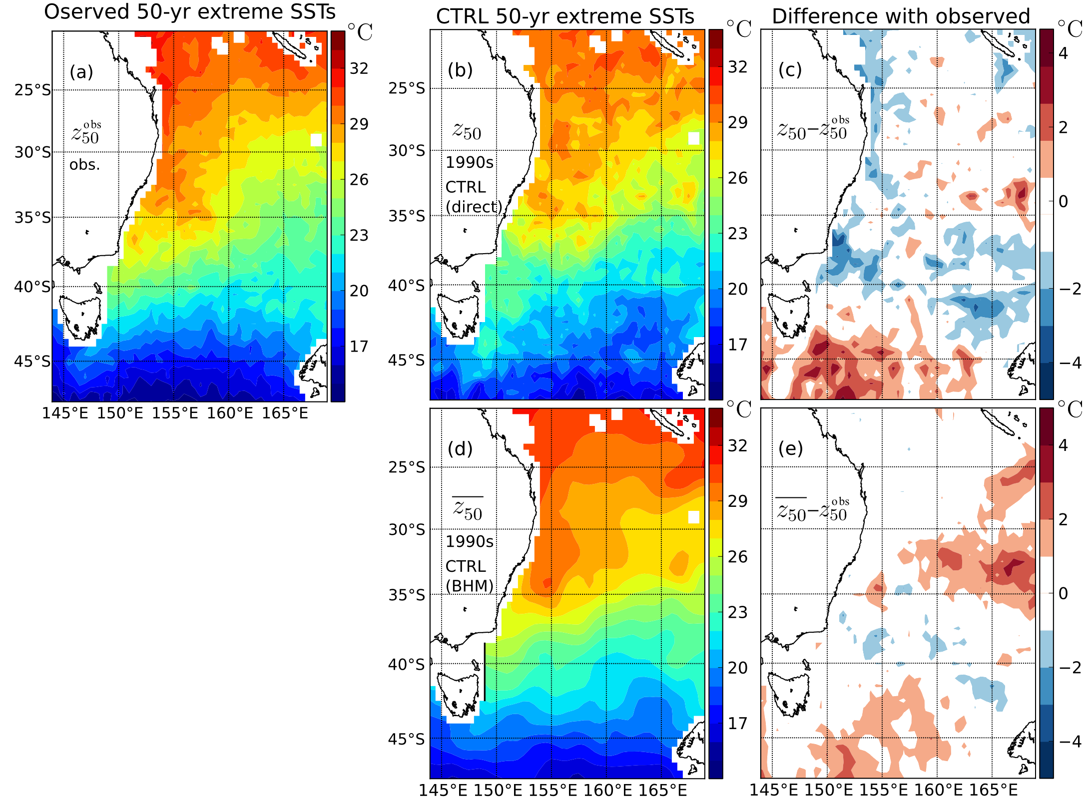
- Results showing the improvement of the Bayesian hierarchical extremes model over the raw ocean model output:

Figure 1: The 50-yr return levels for observed and CTRL simulation sea surface temperatures. The 50-yr return levels were estimated for (a) the observations and (b) the CTRL simulation, using maximum likelihood fits of the Gumbel distribution to the annual maxima and (d) for the CTRL simulation using the Bayesian hierarchical model. (c),(e) The difference between the two estimates of the CTRL simulation extremes and the observations are shown. (click image for hi-res version.)
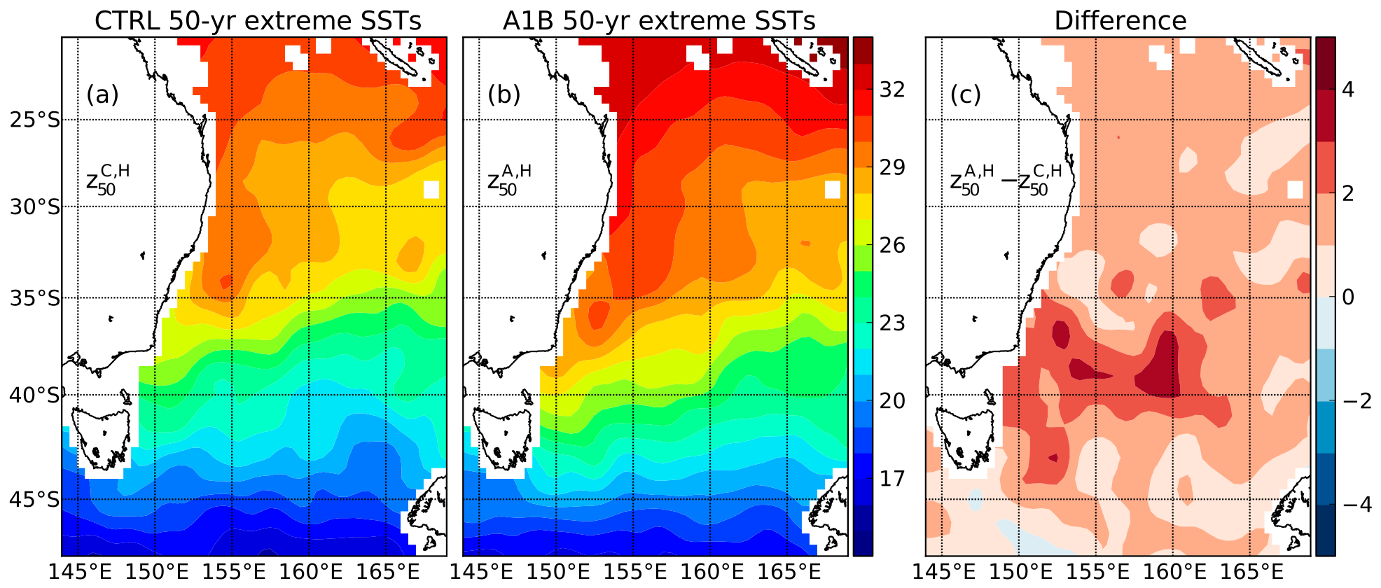
Oliver et al. (Journal of Climate, 2014): Ocean climate extremes have received little treatment in the literature, aside from coastal sea level and temperatures affecting coral bleaching. Further, it is notable that extremes, e.g., temperature and precipitation, are typically not well represented in global climate models. Here, we improve dynamically downscaled ocean climate model estimates of sea surface temperature (SST) extremes in the Tasman Sea off southeastern Australia using satellite remotely-sensed observed extreme SSTs and the simulated marine climate of the 1990s. This is achieved using a Bayesian hierarchical model in which the parameters of an extreme value distribution are modeled by linear regression onto the key marine climate variables, e.g., mean SST, SST variance, etc. We then apply this fitted model, essentially a form of bias correction, to the marine climate projections for the 2060s under an A1B emissions scenario. We show that the extreme SSTs are predicted to increase in the Tasman Sea in a non-uniform way. The 50-year return period extreme SSTs are predicted to increase by up to 2$\dg$C over the entire domain and by up to 4$\dg$C in a hotspot located in the central-western portion of the Tasman Sea, centered at a latitude $\sim$500 km further south than the projected change in mean SST. We show that there is a greater than 50\% chance that annual maximum SSTs will increase by at least 2$\dg$C in this hotspot and that this change is significantly different than that which might be expected due to random chance in an unchanged climate.
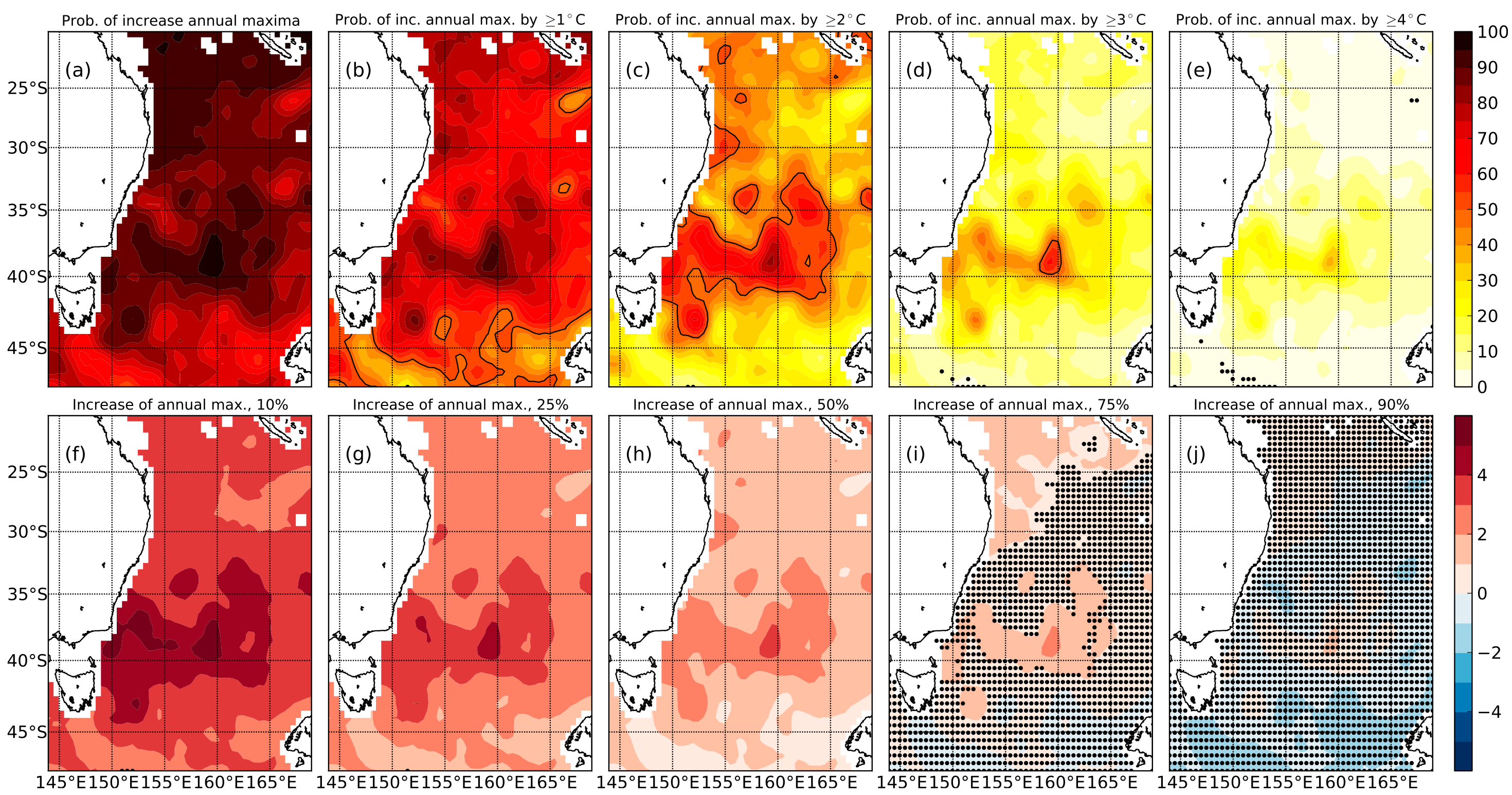
- Since the model is probabilistic in nature we can assign confidence levels to our projections. This is done by testing if the projected changes are greater than what can be expected in an unchanged (1990s) climate, at a specified confidence level:
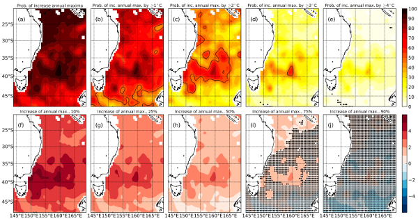
Figure 3: Probabilities of change in annual maxima. (top) Contours indicate (a) the probabilities that the maximum annual SSTs will increase by any amount between the 1990s and 2060s and the probabilities that they will increase by at least (b)–(e) 1 deg. C, 2 deg. C, 3 deg. C, and 4 deg. C. Black dots indicate where these probabilities do not exceed those due to randomness in an unchanged climate. (bottom) Contours indicate the minimum changes in annual maxima estimated with probabilities of (f)–(j) 10%, 25%, 50%, 75%, and 90%. The black dots indicate that the minimum changes do not exceed those due to randomness in an unchanged climate. (click image for hi-res version.)
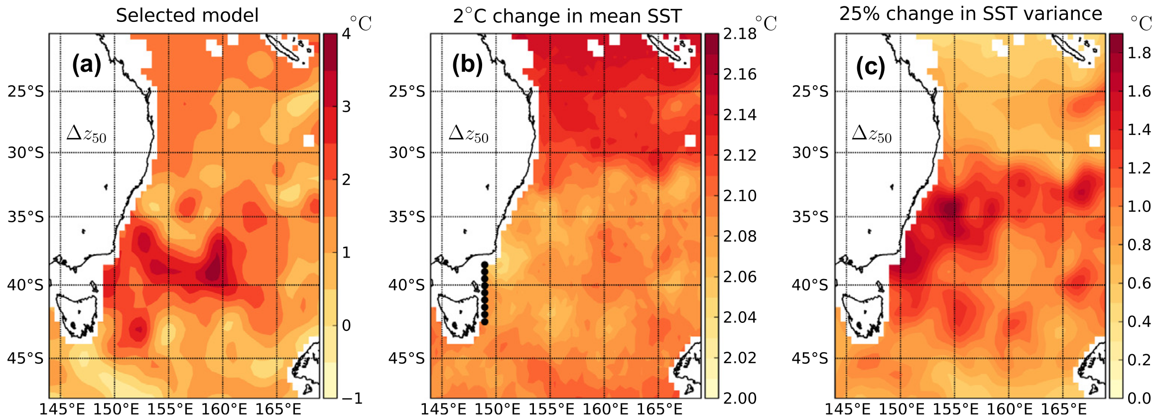
- Since the projected changes in extreme SSTs are informed by changes to the large-scale climate statistics we can use the Bayesian hierarchical model as a "toy model" in order to test the response of the extreme SSTs to prescribed changes in climate, such as a change in the mean or variance of SST:
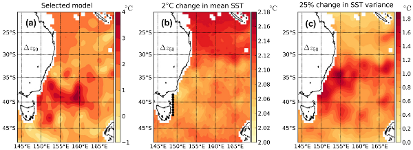
Figure 4: The change in 50-year return levels between the 1990s and the 2060s using the Bayesian hierarchical model for the projected changes in marine climate through 2060 under an A1B emissions scenario (a), for a specified 2 deg. C change in mean SST from the 1990s climate (b), and for a specified 25% change in SST variance from the 1990s climate (c). (click image for hi-res version.)
|